PLOTFOLD⁽⁺⁾

PlotFold displays the optimal and suboptimal secondary structures for an RNA or DNA molecule predicted by MFold.

MFold uses the method of Zuker (see the MFold entry in this manual for more information) to determine optimal and suboptimal secondary structures for an RNA or DNA molecule. MFold writes an output file containing energy matrices that determine all optimal and suboptimal foldings for the molecule. PlotFold reads this output file and displays representations of the optimal and suboptimal foldings.

PlotFold allows you to choose from among eight different representations of the optimal and suboptimal foldings determined by MFold. Each of these options allows you to specify an energy increment, which is the highest deviation in kcal/mole from the computed free energy minimum that a structure can have in order to be plotted. For example, if the predicted optimal folding has a computed free energy of -126.8 kcal/mole, and you select a 6.3 kcal/mole energy increment, then all plotted structures must have calculated free energies no greater than -120.5 kcal/mole (-126.8 + 6.3 = -120.5).

The first two folding representations, the energy dotplot and the p-num plot, plot base pairing information from all secondary structures that have free energies within the energy increment you specify. You can use these displays to determine which regions of the secondary structure prediction are well defined (see the example sessions below).

Energy Dotplot (menu option A)

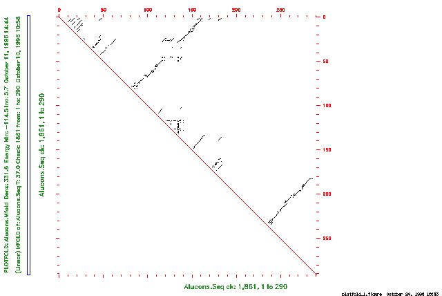
The energy dotplot indicates all of the base pairs involved in all optimal and suboptimal secondary structures within the energy increment you specify. The plot takes the form of a two-dimensional graph where both axes of the graph represent the same RNA sequence. Each point drawn in the graph indicates a base pair between the ribonucleotides whose positions in the sequence are the coordinates of that point on the graph.

P-Num Plot (menu option B)

The p-num plot graphs the amount of variability in pairing at each position in the RNA molecule. For each position of the sequence along the horizontal axis, the height of the plot indicates how many different pairing partners the program finds in all predicted foldings within the energy increment you specify.

The remaining six PlotFold options plot a sampling of specific secondary structures that have calculated free energies within the energy increment you specify. These remaining options all display the same information, but in different forms. Rather than attempting to plot each secondary structure whose computed free energy falls within the energy increment, PlotFold selects representative foldings that are sufficiently different from each other and are still within the specified energy increment. You can specify how different each folding must be from the others with Plotted foldings differ by a distance of at least or in response to the program prompt. To understand the concept of a window size, we must first define the idea of a distance between base pairs in different foldings. The distance between two base pairs, r_(i)-r_(j) and r_(i')-r_(j') is the greater of |i - i'| and |j - j'|. Each listed folding must have at least a window size number of base pairs that are greater than window size distance from the base pairs in any other listed folding.

Each of these five PlotFold options also lets you select the number of structures to plot. Since the number of structures that meet both the energy increment and window size criteria may be less than your selection, fewer secondary structures may actually be plotted.

Circles Plot (menu option C)

The circles plot makes a circular Nussinov plot of a nucleic acid secondary structure. The circular graph represents the sequence as a segment of a circle. You can set the radius and the angular width of one base so that plots of different secondary structures are strictly comparable. Arcs or chords connect paired bases; hairpin, bulge, interior, and multibranched loops are easily seen.

Domes Plot (menu option D)

The domes plot represents a folded nucleotide sequence as a line with elliptical arcs connecting paired bases. This representation has the property that the length of the arc is proportional to the distance (along the primary structure) between the bases; all loops are easily seen.

Mountains Plot (menu option E)

The mountains plot makes a graph that looks like a mountain range. Horizontal striations upon a particular peak are bonds between paired bases, and vertical links between the horizontal striations represent stems.

Squiggles Plot (menu option F)

The squiggles plot is a representation similar to what you might draw by hand; that is, bonds formed between bases are drawn as chords. Bases are shown participating in stems, as well as in hairpin, bulge, interior, and multibranched loops.

Text Output (menu option G)

The text output representation of the nucleic acid secondary structure is similar to the squiggles plot, but you don't need a graphics device to see it. The output is written into a text file that you can view with any text editor. If you exclude a region of the molecule from folding in MFold with either -CLOSedexcise or -OPENexcise, you can view the predicted secondary structures only as text output; do not use any of the graphic plotting options of PlotFold to display the results.

Connect File Output (menu option H)

The Connect file is a base-by-base text output file of optimal and suboptimal RNA or DNA secondary structures. This file can be used as input to several publicly available nucleic acid secondary structure display programs that produce graphical representations of those secondary structures.

The examples below demonstrate three different PlotFold options for the secondary structure representations.

The first example is a session using PlotFold to display an energy dotplot of the secondary structures determined for an Alu consensus RNA sequence in the example session with MFold. The plot indicates all base pairs in all foldings with predicted free energies that are within the increment of the predicted optimal folding energy you specify. If you are reading the Program Manual, the plot from this session is shown in the figure below.

Points drawn in the upper triangular plot represent predicted base pairs in the RNA molecule. For example, a point drawn at position 267 on the vertical axis and position 200 on the horizontal axis indicates a base pair between ribonucleotides 267 and 200 in the sequence.

The plot displays all base pairs in all optimal and suboptimal foldings within the energy increment you specify. On a color plot, you can display base pairs from foldings at different levels of suboptimality with different colors. Black is reserved for base pairs involved in optimal foldings, and other colors are used for base pairs in structures at different levels of suboptimality. The color legend indicates the maximum free energy (in kcal/mole) for each color.

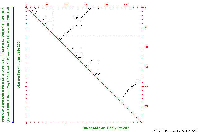
You can use the energy dotplot to determine which regions of the secondary structure prediction are well defined. Well-defined regions are those that have the least variability in all predicted secondary structures. For example, if you draw a vertical line from position 72 on the horizontal axis, and draw a horizontal line from position 72 on the vertical axis, the lines cross only one point on the graph. (If you are reading the Program Manual, this is shown in the figure below.) This means that when the ribonucleotide at position 72 is paired, it has the same pairing partner (at position 92) in all predicted optimal and suboptimal foldings within 6.3 kcal/mole of the computed optimal folding.

The second example is a session using PlotFold to display a p-num plot of the secondary structures determined for an Alu consensus RNA sequence in the example session with MFold. This plot shows the amount of variability in pairing at each position in the sequence in all predicted foldings within the increment of the optimal folding energy you specify.

If you are reading the Program Manual, the plot from this session is shown in the figure below.

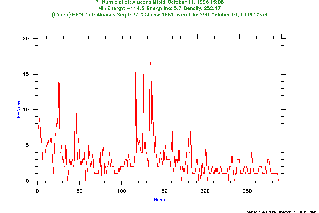
For each position of the sequence along the horizontal axis, the height of the plot indicates how many different pairing partners are found in all predicted optimal and suboptimal foldings within the energy increment you specify. You can use this information to help determine which regions of the secondary structure prediction are well defined. For example, the ribonucleotide at position 135 forms base pairs with 18 different bases in all computed secondary structures within 6.3 kcal/mole of the optimal folding. This great variability indicates that the pairing at this position may not be reliably determined. On the other hand, the ribonucleotide at position 36 forms no base pairs in all secondary structures within 6.3 kcal/mole of the computed optimal folding. This nucleotide may be reliably determined to be single-stranded in the "correct" folding.

The last example is a session using PlotFold to display mountains plots of optimal and suboptimal foldings determined for an Alu consensus RNA sequence in the example session with MFold. The program plots representative secondary structures that satisfy the energy increment and window size criteria you specify.

The plot from this session is shown in the figure below.

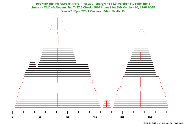
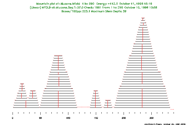
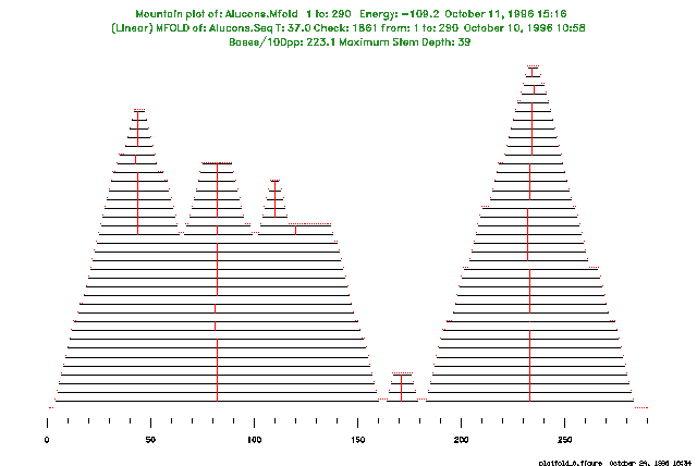
Note that, although we requested 25 structure plots by default, the program plots only the three different structures that satisfy both the energy increment and window size criteria.

PlotFold accepts the energy matrix output file from MFold as input. This file cannot be read by eye. The energy matrix output files created by MFold in Version 7 of the Wisconsin Package cannot be read as input by PlotFold in later versions of the Wisconsin Package. To read Version 7 MFold output files, use the program OldPlotFold.

MFold predicts optimal and suboptimal secondary structures for an RNA or DNA molecule using the most recent energy minimization method of Zuker. PlotFold displays the optimal and suboptimal secondary structures for an RNA or DNA molecule predicted by MFold.

StemLoop finds all possible stems (inverted repeats) above some minimum quality that you can set, but StemLoop cannot recognize a structure with gaps (bulge loops or uneven bifurcation loops). The stems can be plotted with DotPlot.

If you exclude a region of the RNA molecule from folding in MFold with either -CLOSedexcise or -OPENexcise, you can display the predicted secondary structures using only the text output option (menu option G); do not use any of the graphic plotting options of PlotFold to display the results.

In Dr. Zuker's original program, you can select any base pair in the energy dotplot and the program then computes the folding of lowest free energy that includes that base pair. The GCG version of MFold currently does not include this feature.

PlotFold is an adaptation of part of the mfold package by Zuker and Jaeger (see the MFold entry in the Program Manual) that incorporates GCG routines to display representations of RNA secondary structures.

We thank Dr. Zuker, not only for making his work available to GCG, but also for helping us incorporate his work into the Wisconsin Package^(TM).

The idea of representing nucleic acid secondary structures with circular graphs (menu option C) comes from the work of Nussinov et al. (SIAM Journal of Applied Math. 35; 68-82 (1978)). Circular graphs were also used to illustrate the argument for Zuker's original paper describing the prediction of RNA secondary structure by energy minimization (Nucl. Acids Res. 9(1); 133-148 (1981)). John Devereux and Yonah D. Karp wrote the code for the GCG implementation of a circular graph display. William Winsborough worked out the trigonometry for this implementation.

The idea of representing nucleic acid secondary structures with elliptical arcs that intersect with a straight line (menu option D) was proposed by Professor Paul Kaesberg (unpublished) as an extension to the circular graph representation. A program to draw this elliptical representation was first written for the IBM PC by Professor Claire Rinehart of the University of Western Kentucky. John Devereux wrote the code for the GCG implementation.

The idea of a mountains display (menu option E) of nucleic acid secondary structures comes from Hogeweg and Hesper, Nucl. Acids Res. 12; 67-74 (1984). The GCG implementation of this mountains display was written by Verne A. Luckow and Yonah D. Karp.

The squiggles display (menu option F) originates with the work of Osterburg and Sommer (Comput. Programs in Biomed. 13; 101-109 Figure 7 (1981)). The subroutine DRWFLD was taken from a FORTRAN translation of their program and extensively revised by Verne Luckow and Yonah D. Karp.

GCG is allowed to distribute a GCG-compatible implementation of MFold under a license agreement with the National Research Council of Canada, Institute for Biological Sciences, Ottawa, Canada, K1A 0R6 (613)-993-4830. The copyright to MFold, however, belongs to the Government of Canada. If you use MFold for published research, cite Dr. Zuker's Science paper (see the MFold entry in the Program Manual for the appropriate reference). Any communication of the MFold program must be approved by the National Research Council of Canada.

You can set the parameters listed below from the command line. For more information, see "Using Program Parameters" in Chapter 3, Using Programs in the User's Guide.

Type of Plot

energy dotplot
p-num plot
circles
domes
mountains
squiggles

choose the type plot to display (a squiggles plot shows the stems and loops).

Energy Dotplot

Set the energy increment at which to plot structures or base pairs

sets the energy increment (in kcal/mole) at which to plot base pairs. PlotFold plots all base pairs involved in all predicted secondary structures whose computed minimum free energies differ by no more than this increment from the computed minimum free energy of the optimal structure.

Color levels of suboptimality

sets the number of colors used to plot the base pairs on a color graphics device. Each base pair is colored according to the minimum free energy of all predicted structures containing that base pair, as described in the plot legend. Specifying multiple colors allows you to distinguish base pairs from structures at different levels of suboptimality in a single graph. This setting applies to energy dotplot displays only.

Symbol to Plot

point
square
octagon
triangle
+
X
diamond
*
|

defines a centered symbol to be used for every point. The available symbols are Point=0, Square=1, Octogon=2, Triangle=3, +=4, X=5, Diamond=6, *=7, and |=8. This option applies to energy dotplots only.

Set symbol height

defines the height for symbols (other than points) in units of one percent of the plotter's vertical axis (one platen unit). This option applies to energy dotplots only.

Draw an axis of symmetry

suppresses drawing an axis of symmetry along the central diagonal of the plot. This option applies to energy dotplots only.

P-Num Plot

Set the energy increment at which to plot structures or base pairs

sets the energy increment (in kcal/mole) at which to plot base pairs. PlotFold plots all base pairs involved in all predicted secondary structures whose computed minimum free energies differ by no more than this increment from the computed minimum free energy of the optimal structure.

Circles Plot

Set the energy increment at which to plot structures or base pairs

For engery dotplots and p-num plots: sets the energy increment (in kcal/mole) at which to plot base pairs. PlotFold plots all base pairs involved in all predicted secondary structures whose computed minimum free energies differ by no more than this increment from the computed minimum free energy of the optimal structure.

For other plots: sets the energy increment (in kcal/mole) at which to save secondary structures. PlotFold saves representative structures whose computed minimum free energies differ by no more than this increment from the computed minimum free energy of the optimal structure.

Maximum number of structures to display

specifies the maximum number of predicted optimal and suboptimal secondary structures to save.

Plotted foldings differ by a distance of at least

specifies the minimum difference among saved secondary structures in terms of a window size. To understand the concept of a window size, we must first define the idea of a distance between base pairs in different folding. The distance between two base pairs, r_(i)-r_(j) and r_(i')-r_(j') is the greater of |i - i'| and |j - j'|. Each saved secondary structure must have at least a window size number of base pairs that are greater than window size distance from the base pairs in any other saved structure.

Set degrees of arc given to each base

sets the degrees of arc given to each base in the plot. This setting applies to the circles plot only.

Radius of circle

sets the radius of the circle plot. This setting applies to the circles plot only.

Display the sequence

prints the sequence around the circumference.

Connect paired bases with chords instead of circles

connects bases with straight lines. Normally the circles plot uses circular segments to connect bases that are paired.

Domes Plot

Set the energy increment at which to plot structures or base pairs

For engery dotplots and p-num plots: sets the energy increment (in kcal/mole) at which to plot base pairs. PlotFold plots all base pairs involved in all predicted secondary structures whose computed minimum free energies differ by no more than this increment from the computed minimum free energy of the optimal structure.

For other plots: sets the energy increment (in kcal/mole) at which to save secondary structures. PlotFold saves representative structures whose computed minimum free energies differ by no more than this increment from the computed minimum free energy of the optimal structure.

Maximum number of structures to display

specifies the maximum number of predicted optimal and suboptimal secondary structures to save.

Plotted foldings differ by a distance of at least

specifies the minimum difference among saved secondary structures in terms of a window size. To understand the concept of a window size, we must first define the idea of a distance between base pairs in different folding. The distance between two base pairs, r_(i)-r_(j) and r_(i')-r_(j') is the greater of |i - i'| and |j - j'|. Each saved secondary structure must have at least a window size number of base pairs that are greater than window size distance from the base pairs in any other saved structure.

Display the sequence

prints the sequence itself below the number line.

Mountains Plot

Set the energy increment at which to plot structures or base pairs

For engery dotplots and p-num plots: sets the energy increment (in kcal/mole) at which to plot base pairs. PlotFold plots all base pairs involved in all predicted secondary structures whose computed minimum free energies differ by no more than this increment from the computed minimum free energy of the optimal structure.

For other plots: sets the energy increment (in kcal/mole) at which to save secondary structures. PlotFold saves representative structures whose computed minimum free energies differ by no more than this increment from the computed minimum free energy of the optimal structure.

Maximum number of structures to display

specifies the maximum number of predicted optimal and suboptimal secondary structures to save.

Plotted foldings differ by a distance of at least

specifies the minimum difference among saved secondary structures in terms of a window size. To understand the concept of a window size, we must first define the idea of a distance between base pairs in different folding. The distance between two base pairs, r_(i)-r_(j) and r_(i')-r_(j') is the greater of |i - i'| and |j - j'|. Each saved secondary structure must have at least a window size number of base pairs that are greater than window size distance from the base pairs in any other saved structure.

Display the sequence

replaces the dots around the plot with letters showing the bases. -NOSHOwseq is the default.

Squiggles Plot

Set the energy increment at which to plot structures or base pairs

For engery dotplots and p-num plots: sets the energy increment (in kcal/mole) at which to plot base pairs. PlotFold plots all base pairs involved in all predicted secondary structures whose computed minimum free energies differ by no more than this increment from the computed minimum free energy of the optimal structure.

For other plots: sets the energy increment (in kcal/mole) at which to save secondary structures. PlotFold saves representative structures whose computed minimum free energies differ by no more than this increment from the computed minimum free energy of the optimal structure.

Maximum number of structures to display

specifies the maximum number of predicted optimal and suboptimal secondary structures to save.

Plotted foldings differ by a distance of at least

specifies the minimum difference among saved secondary structures in terms of a window size. To understand the concept of a window size, we must first define the idea of a distance between base pairs in different folding. The distance between two base pairs, r_(i)-r_(j) and r_(i')-r_(j') is the greater of |i - i'| and |j - j'|. Each saved secondary structure must have at least a window size number of base pairs that are greater than window size distance from the base pairs in any other saved structure.

Display the sequence

labels the bases. This setting does not apply to energy dotplots and p-num plots.

Text Output

Set the energy increment at which to plot structures or base pairs

For engery dotplots and p-num plots: sets the energy increment (in kcal/mole) at which to plot base pairs. PlotFold plots all base pairs involved in all predicted secondary structures whose computed minimum free energies differ by no more than this increment from the computed minimum free energy of the optimal structure.

For other plots: sets the energy increment (in kcal/mole) at which to save secondary structures. PlotFold saves representative structures whose computed minimum free energies differ by no more than this increment from the computed minimum free energy of the optimal structure.

Maximum number of structures to display

specifies the maximum number of predicted optimal and suboptimal secondary structures to save.

Plotted foldings differ by a distance of at least

specifies the minimum difference among saved secondary structures in terms of a window size. To understand the concept of a window size, we must first define the idea of a distance between base pairs in different folding. The distance between two base pairs, r_(i)-r_(j) and r_(i')-r_(j') is the greater of |i - i'| and |j - j'|. Each saved secondary structure must have at least a window size number of base pairs that are greater than window size distance from the base pairs in any other saved structure.

Connect File Output

Set the energy increment at which to plot structures or base pairs

For engery dotplots and p-num plots: sets the energy increment (in kcal/mole) at which to plot base pairs. PlotFold plots all base pairs involved in all predicted secondary structures whose computed minimum free energies differ by no more than this increment from the computed minimum free energy of the optimal structure.

For other plots: sets the energy increment (in kcal/mole) at which to save secondary structures. PlotFold saves representative structures whose computed minimum free energies differ by no more than this increment from the computed minimum free energy of the optimal structure.

Maximum number of structures to display

specifies the maximum number of predicted optimal and suboptimal secondary structures to save.

Plotted foldings differ by a distance of at least

specifies the minimum difference among saved secondary structures in terms of a window size. To understand the concept of a window size, we must first define the idea of a distance between base pairs in different folding. The distance between two base pairs, r_(i)-r_(j) and r_(i')-r_(j') is the greater of |i - i'| and |j - j'|. Each saved secondary structure must have at least a window size number of base pairs that are greater than window size distance from the base pairs in any other saved structure.

The parameters below apply to all Wisconsin Package graphics programs. These and many others are described in detail in Chapter 5, Using Graphics of the User's Guide.

Printed: January 13, 1999 6:27 (1162)